


Lidar measurements of atmospheric depolarization can be used to
distinguish between liquid and solid phases of water in the
atmosphere [36,37,38].
The quantity to describe the degree of polarization is
the linear depolarization ratio 

where  and
and  are the measured perpendicular and parallel
backscatter intensities in respect to the transmitter polarization
axis.
The backscatter signal of a linearly polarized laser beam from
spherical particles is totally linearly polarized
(
are the measured perpendicular and parallel
backscatter intensities in respect to the transmitter polarization
axis.
The backscatter signal of a linearly polarized laser beam from
spherical particles is totally linearly polarized
( ). The particles can be assumed to be spherical in
case of wet haze, fog, cloud droplets, and small raindrops.
The depolarization of the pure molecular atmosphere is
nonzero, because of the anisotropy of the air, and therefore
a 0.37--0.4 % depolarization for the Cabannes line is expected
[39,40].
The depolarization of the molecular return that includes the Cabannes
line and the rotational Raman lines is
). The particles can be assumed to be spherical in
case of wet haze, fog, cloud droplets, and small raindrops.
The depolarization of the pure molecular atmosphere is
nonzero, because of the anisotropy of the air, and therefore
a 0.37--0.4 % depolarization for the Cabannes line is expected
[39,40].
The depolarization of the molecular return that includes the Cabannes
line and the rotational Raman lines is  1.5% [40].
If particles are nonspherical (as ice crystals, snow flakes or
dust particles) or
if the backscatter signal has a multiple scattering contribution,
the backscattered signal contains a cross-polarized component
(
1.5% [40].
If particles are nonspherical (as ice crystals, snow flakes or
dust particles) or
if the backscatter signal has a multiple scattering contribution,
the backscattered signal contains a cross-polarized component
( ).
A specular reflection from a oriented ice crystal layer
provides a small depolarization, which therefore can
be misinterpreted as the backscatter signal from a water cloud,
but the off vertical pointing direction of the HSRL is
expected to prevent this.
).
A specular reflection from a oriented ice crystal layer
provides a small depolarization, which therefore can
be misinterpreted as the backscatter signal from a water cloud,
but the off vertical pointing direction of the HSRL is
expected to prevent this.
Lidar studies of atmospheric polarization have been traditionally based on a technique, where a linearly polarized laser beam is sent to the atmosphere and the received polarization components are separated by a polarization cube and detected by a pair a photomultiplier tubes, one for each polarization component. This method requires a precise calibration of the receiver in order to avoid the problems due to differences between channels in optics, and in photomultiplier sensitivity.
In the new HSRL (see Figs. 5 and {6),
the polarization measurements are made by using one
transmitter laser and one detector for both polarization components.
The transmitted laser beam is linearly polarized, and for polarization
measurements the polarization of the transmitted laser beam is rotated by
90 degrees on alternative laser pulses by a Pockels cell. In the
receiver, the signal parallel to the transmitter polarization axis
and the signal perpendicular to that are separated and cleaned by
a polarization cube pair.
Since the polarization of the transmitted laser shot alternates between two
subsequent laser shots, the same detector can accurately measure
both polarization components and therefore no calibration of the
receiver is required. The 250  s time separation between
laser pulses insures, that both depolarization components are measured
from the same atmospheric scatterers. The depolarization variations as
a function of field of view can be studied with the new WFOV-channel.
The effects of specular reflection from a horizontally oriented
crystal layer are minimized
by tilting the receiver by 4 degrees
from the zenith.
With the HSRL, separate measurements of aerosol and molecular
depolarizations can be made.
s time separation between
laser pulses insures, that both depolarization components are measured
from the same atmospheric scatterers. The depolarization variations as
a function of field of view can be studied with the new WFOV-channel.
The effects of specular reflection from a horizontally oriented
crystal layer are minimized
by tilting the receiver by 4 degrees
from the zenith.
With the HSRL, separate measurements of aerosol and molecular
depolarizations can be made.
Depolarization measurements are affected by presence of multiple
scattering when a lidar is used to probe dense clouds.
Because the amount of detected multiple scattering is dependent
from the cloud particle size, range from the cloud, optical
depth of the cloud, and the field of view of the system,
typical systems with 1-5 mrad field of views
have difficulties separating
between water and ice for dense clouds. In order to
separate between water and ice for optically thick clouds, the
HSRL uses a 160  rad field of view for the spectrometer
channels.
rad field of view for the spectrometer
channels.
Figure 27 represents an example of the multiple scattering effect on the measured depolarization. Figure 27.a. shows the measured energy and range square corrected signals from a supercooled water cloud with ice precipitation. For the WFOV-channels, 0.22, 0.65, 1.1, and 1.6 mrad field of views are used. The WFOV-channel measurements are then compared to the measurements of the 0.16 mrad field of view channels. The amount of multiple scattering in the signal is calculated from the ratio of the WFOV-signal to the signal simultaneously measured with the narrow field of view channel (see Figure 27.b.). Figure 27.c shows the depolarization ratios for different field of views and the Figure 27.d shows the ratio of the WFOV depolarization to the narrow field of view depolarization. For the optically thin ice crystal precipitation layer, the change in depolarization as a function of field of view is hardly noticeable. The change from ice to water shows up as a drop in the depolarization ratio. All field of views show a low depolarization for the water cloud base but as soon as the signal penetrates deeper into the cloud, an increase in the depolarization as a function of field of view can be observed. Inside 300 m the multiple scattering effects in the cloud will increase the depolarization of the larger field of views up to the level which is comparable with the observed ice crystal depolarization and therefore, the separation between ice and water becomes impossible. The low values of depolarization observed with the narrow field of view channel and with the smallest WFOV field of view show that the narrow field of view effectively suppresses the effects of multiple scattering. Therefore, the HSRL signals from these field of views can be used to separate between ice and water clouds even for optically thick clouds. On the other hand, information from depolarization and signal strength variations as a function of field of view can be used to verify multiple scattering calculations.
Theoretically, the depolarization of the spherical dropplets should be
zero, but the depolarization ratios observed for the water cloud at 5.5 km
is  2 %. In the cases of water clouds with an ice crystal precipitation,
the non-zero values of depolarization ratio can be explained by the presence
of ice. Because the water cloud is precipitating ice, there has to be
some ice mixed with water in the cloud.
The scattering from the cloud base
is
2 %. In the cases of water clouds with an ice crystal precipitation,
the non-zero values of depolarization ratio can be explained by the presence
of ice. Because the water cloud is precipitating ice, there has to be
some ice mixed with water in the cloud.
The scattering from the cloud base
is  20 times larger than signal from ice crystal precipitation.
Based on this ratio,
20 times larger than signal from ice crystal precipitation.
Based on this ratio,
 2 %
(
2 %
( 1/20 x ice depolarization of 40 %)
depolarization for the cloud base depolarization can
be expected due to the presence of ice crystals with
1/20 x ice depolarization of 40 %)
depolarization for the cloud base depolarization can
be expected due to the presence of ice crystals with  40 % depolarization.
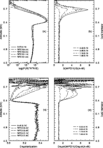
Figure 27: Effects of multiple scattering on depolarization in
the backscatter return from a water cloud at 5.5 km with
ice crystal precipitation between 4.5 and 5.3 km. Data obtained on
November 11, 1993 02:04-02:14 UT.
(a) Measured signals.
(b) Ratios of measured WFOV signals to 0.16 mrad field of view signal.
(c) Measured depolarization ratios. The cloud base depolarization
of the smallest field of view at 5.4 km is  2 %.
(d) Ratios of the measured WFOV depolarizations to the depolarization of
the 0.16 mrad field of view channel.
2 %.
(d) Ratios of the measured WFOV depolarizations to the depolarization of
the 0.16 mrad field of view channel.
The capability of the HSRL to distinguish between aerosol and molecular scattering allows separate polarization measurements. This is important when layers with a low aerosol content are studied. The effects of the molecular scattering on the observed depolarization can be seen by comparing the raw and inverted aerosol depolarization ratios. For the cases where the amount of aerosol scatterers is small, the signal from molecular scattering dominates the depolarization picture (see Figure 23). Therefore, aerosol depolarizations similar to the molecular depolarization can be seen and also parts of the cirrus cloud and ice crystal precipitation show depolarization ratios which are close to the depolarization of the supercooled water or mixture of ice and water (green areas in the raw aerosol depolarization RTI). After inversion a clear difference in the depolarizations is seen: the depolarization of the low level aerosols is better defined and the depolarization of the cirrus shows that the cloud contains pure ice crystals (Figure 24). Therefore, a clear separation between ice and water can be based to the depolarization ratios calculated from the inverted aerosol profiles. The effect of the inversion to the depolarization ratio is also visible from the Figures 28 -- 29.
The profile of the raw aerosol depolarization shows the depolarization of the combined aerosol+molecular channel and therefore, it shows the depolarization ratio which is seen with a conventional single channel lidar. The raw molecular depolarization contains the depolarization component of the aerosol cross talk together with the molecular depolarization. In the same figure, the separated aerosol and molecular signals are shown with the inverted aerosol and molecular depolarizations. Figure 28 shows a two layer water cloud with an ice crystal precipitation. The peaks of the water clouds are observed at 5.2 and 5.6 km and the corresponding low depolarization values are 1--2 %. A small increase in the depolarization with penetration depth is observed. The values of raw depolarization of the ice crystal precipitation are close to those of water and ice mixture, but the inverted depolarization ratios show a clear ice depolarization. After inversion the increase in aerosol depolarization at 2--3.7 km is also very clear. The Figure 29 shows a water cloud layer at 5.4 km with a more dense ice crystal precipitation. With increased backscatter signal from ice, the value of raw depolarization ratio indicates clear ice and therefore the effects of molecular depolarization do not show up so clearly, eventhough a change in depolarization ratio is observed after the inversion.
The depolarization observed in the clear air is 0.7--0.8 %,
when the observations are made without the low resolution etalons.
When the low resolution etalons are used, the depolarization is
0.55--0.6 %. The expected value for the molecular depolarization
of the Cabannes line is  0.4
and
0.4
and  1.44 for the Cabannes
line[39,40] and rotational Raman lines [40].
The HSRL observations show a 1.5 % depolarization for the signal from
the rotational Raman lines and Cabannes line.
Because the system filter bandpass admits a small fraction of the
rotational Raman lines (75 % depolarization) and
simultaneously blocks part of the Cabannes line,
the molecular depolarization value measured by the HSRL is
larger than the expected Cabannes line depolarization. The
amount of transmitted rotational Raman signal is temperature dependent.
A model to calculate the expected depolarization was written.
This model includes the rotational Raman spectrum for nitrogen
and oxygen, molecular spectrum including effects of Brillouin scattering, and
spectral transmissions of different filters. The polarization
that correspond to different atmospheric temperatures can be
calculated.
The ratio of
rotational Raman signal to Rayleigh signal is chosen so,
that a 1.44 % depolarization for the clear air is observed.
These calculations show, that a 0.56 --0.62 % depolarization
is expected for the case where no low resolution etalons were used.
A 0.402 --0.425 % depolarization is expected, when
one or two etalon are used. The depolarization observed with
the HSRL are larger than the expected values. The cause of the additional
depolarization in the HSRL measurements is currently unknown.
1.44 for the Cabannes
line[39,40] and rotational Raman lines [40].
The HSRL observations show a 1.5 % depolarization for the signal from
the rotational Raman lines and Cabannes line.
Because the system filter bandpass admits a small fraction of the
rotational Raman lines (75 % depolarization) and
simultaneously blocks part of the Cabannes line,
the molecular depolarization value measured by the HSRL is
larger than the expected Cabannes line depolarization. The
amount of transmitted rotational Raman signal is temperature dependent.
A model to calculate the expected depolarization was written.
This model includes the rotational Raman spectrum for nitrogen
and oxygen, molecular spectrum including effects of Brillouin scattering, and
spectral transmissions of different filters. The polarization
that correspond to different atmospheric temperatures can be
calculated.
The ratio of
rotational Raman signal to Rayleigh signal is chosen so,
that a 1.44 % depolarization for the clear air is observed.
These calculations show, that a 0.56 --0.62 % depolarization
is expected for the case where no low resolution etalons were used.
A 0.402 --0.425 % depolarization is expected, when
one or two etalon are used. The depolarization observed with
the HSRL are larger than the expected values. The cause of the additional
depolarization in the HSRL measurements is currently unknown.
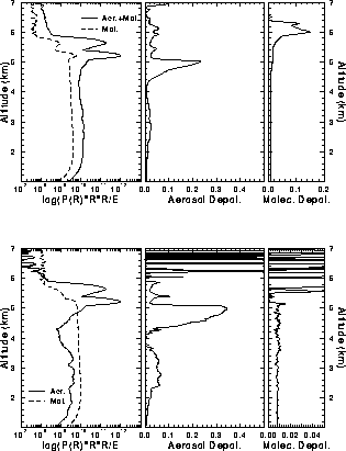
Figure 28: Raw and inverted depolarization ratios of clear atmosphere with
ice crystal precipitation and two water cloud layers above it
(November 11,1993 01:35-01:47 UT).
The upper set shows the raw aerosol and raw molecular profiles together
with the depolarizations.
The lower set shows the inverted profiles
with the inverted depolarizations.
The water clouds are observed at 5.2 and 5.6 km
altitudes. The low water cloud depolarization values can be
observed from the aerosol depolarization figures. The small
increase in water cloud depolarization as a function of penetration
depth is due to the multiple scattering.
The weak signal from the ice crystal precipitation is
visible 4.3-5.1 km. Because of the low ice crystal content,
the raw depolarization ratios of the ice crystal precipitation shows
values that would indicate mixed phase, but after the
inversion a clear ice crystal depolarization is visible. The
clear air aerosol depolarization is less than 6%. The observed molecular
depolarization is 0.8 %.
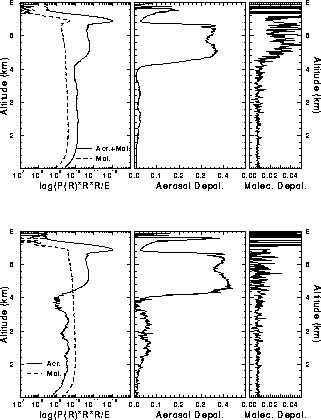
Figure 29: Raw and inverted depolarization ratios of a thin cirrus cloud
and a thin water cloud with an ice crystal precipitation
(November 11,1993 01:55-02:01 UT).
The upper set shows the raw aerosol and molecular profiles along
with the raw depolarization ratios. The lower set shows the inverted profiles
with the inverted depolarization ratios. The water cloud at 5.5 km has
a low depolarization value  1.5% at the cloud base and
it increases towards the cloud top due to the multiple scattering.
The dense ice crystal precipitation is visible between 4 and 5.4 km.
Because the ice crystal content of the precipitation is large
compared to the molecular backscatter, only small difference
between raw and inverted aerosol depolarizations is observed.
The raw molecular depolarization shows a small increase for the
cloud, but after the inversion a constant 0.8% depolarization is observed.
1.5% at the cloud base and
it increases towards the cloud top due to the multiple scattering.
The dense ice crystal precipitation is visible between 4 and 5.4 km.
Because the ice crystal content of the precipitation is large
compared to the molecular backscatter, only small difference
between raw and inverted aerosol depolarizations is observed.
The raw molecular depolarization shows a small increase for the
cloud, but after the inversion a constant 0.8% depolarization is observed.
The depolarization data for cirrus clouds obtained between
August and November 1993 have been
analyzed. A summary of the observed depolarization ratios as
a function of temperature are presented in Figure 30.
In this study only clouds with scattering
ratios greater than 0.5 were used. This was made in order to fully
separate cloud depolarizations from noisy clear air depolarizations.
The values of clear air depolarizations are low and affected by
the photon counting statistics.
Because the HSRL measurements have shown, that the
scattering ratios of clear air aerosol and stratospheric aerosols
can exceed values 1-3, the use of the scattering ratio of 0.5
does not guarantee a clear separation between clouds and
clear air aerosols.
On the other hand, the scattering ratios
of the cirrus clouds can be below 1. Therefore,
a visual separation between cirrus clouds and clear air aerosols
is made and only the cloud altitudes are included to the study.
In this study, 2 min averaging times for the data were used.
By using a short averaging time, the errors
due to temporal changes of the atmosphere were minimized.
The atmospheric temperatures were obtained from radiosonde measurements
and temperature intervals of 5  C were used.
Water clouds at cirrus cloud altitudes were separated from ice
clouds based on the depolarization ratio values. Clouds with
depolarization ratio values less than 15 % were classified
as water clouds.
C were used.
Water clouds at cirrus cloud altitudes were separated from ice
clouds based on the depolarization ratio values. Clouds with
depolarization ratio values less than 15 % were classified
as water clouds.
The high depolarization values of the cirrus
clouds are
easily separable from the water cloud depolarizations.
The average cirrus cloud depolarization varies from
33% to 41% showing
an increase towards
the colder temperatures. Part of this can be expected to be from
different shape, size, and orientation of the ice crystals at
different temperatures [41,42]. The size and shape of the ice
crystals have been found to be different at different temperatures
and the crystals have been found to have a preferred orientation.
A similar increase in cloud depolarization towards colder temperature
was observed by Platt et al. [43]. His study was made for
midlatitude and tropical cirrus and the depolarization
values for temperatures from -30 C to -10
  C were lower,
ranging from
C were lower,
ranging from  0.15 to
  0.25.
The cirrus cloud depolarizations measured with the HSRL do
not show any depolarization values below 20% for the
temperatures from -30 to -10
0.25.
The cirrus cloud depolarizations measured with the HSRL do
not show any depolarization values below 20% for the
temperatures from -30 to -10  C.
The system used
by Platt had a 2.5 mrad field of view, and the low depolarization
values are possibly caused by multiple scattering from
water clouds. The HSRL measurements have shown that when the depolarization
of a water cloud is measured with a system with
C.
The system used
by Platt had a 2.5 mrad field of view, and the low depolarization
values are possibly caused by multiple scattering from
water clouds. The HSRL measurements have shown that when the depolarization
of a water cloud is measured with a system with
 1.0 mrad field of view, the effects of multiple scattering
are large enough to cause depolarization values of
1.0 mrad field of view, the effects of multiple scattering
are large enough to cause depolarization values of  20%, and
therefore the separation between water and ice becomes impossible.
Also the HSRL measurements show a substantial probability of observing
water at temperatures
from -30 to 0
20%, and
therefore the separation between water and ice becomes impossible.
Also the HSRL measurements show a substantial probability of observing
water at temperatures
from -30 to 0  C.
C.
In 45% of the cases simultaneous observations
of water cloud layers at the cirrus cloud altitudes were made.
The Figure 30 shows,
that supercooled water clouds at cirrus cloud altitudes
are found at temperatures as low as -35  C.
Above 0
C.
Above 0 C temperature the low depolarization values indicate
pure water, and the presence of cirrus disappears.
The water cloud depolarizations are below 10 % and
they contain the effects of multiple scattering.
When the same clouds are studied with a NOAA-11 or NOAA-12 satellite,
the simultaneous
appearance of the water and ice cannot be noticed.
On the satellite measurements, the cloud types are separated
by using the information on the temperature.
Therefore, if satellite data is used for cirrus
optical depth studies, a supercooled water cloud layer mixed with ice
cannot be easily separated and water will
increase the optical depth value determined for the cirrus cloud.
The depolarization ratio
knowledge of the cloud measured with a lidar can be used
to separate the water from ice and therefore separate optical
depth measurements for both constituents can be performed.
C temperature the low depolarization values indicate
pure water, and the presence of cirrus disappears.
The water cloud depolarizations are below 10 % and
they contain the effects of multiple scattering.
When the same clouds are studied with a NOAA-11 or NOAA-12 satellite,
the simultaneous
appearance of the water and ice cannot be noticed.
On the satellite measurements, the cloud types are separated
by using the information on the temperature.
Therefore, if satellite data is used for cirrus
optical depth studies, a supercooled water cloud layer mixed with ice
cannot be easily separated and water will
increase the optical depth value determined for the cirrus cloud.
The depolarization ratio
knowledge of the cloud measured with a lidar can be used
to separate the water from ice and therefore separate optical
depth measurements for both constituents can be performed.
The initial measurements have shown that the HSRL is capable of measuring cirrus cloud particle sizes. These measurements together with phase function measurements can be used for further studies of the cloud particle size effects on the depolarization ratio [26].
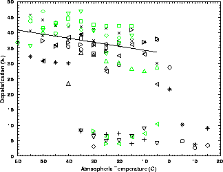
Figure 30: Cirrus cloud and supercooled water cloud depolarization
as a function of temperature observed between August 2 and November 11, 1993.
The depolarization values below 10% are indication
of water clouds and higher depolarization values indicate the presence of ice.