Return to the Publications.
Return to the Index.
Given a temperature profile and vertical distribution of gaseous constituents in a clear atmosphere, one can derive the radiance if the spectroscopic properties of the gas are also known. For monochromatic radiation, the differential transmissivity through the atmosphere is determined by
where
|
| = | atmospheric transmission from |
|
| = | absorption of
atmospheric constituent x, m |
|
| = | wavenumber, cm |
| g | = | gravitational acceleration, m s |
|
| = | mixing ratio of
constituent x, g kg |
| p | = | pressure at given level, hPa. |
Atmospheric pressure units are often expressed in mb, and are equivalent to hPa.
The general radiative transfer equation (RTE) for downwelling spectral radiance in a clear atmosphere is described by the relation
where
represents the Planck radiance, mW (m![]() sr cm
sr cm![]() )
)![]() ;
;
![]()
is the differential transmission over the pressure layers;
|
| = | AERI measured downwelling column radiance, |
| mW (m | ||
| T(p) | = | temperature at pressure level p, K; |
| h | = | Planck's constant, J s; |
| c | = | speed of light, m s |
| k | = | Boltzmann's constant, J K |
and the integral limits, ![]() and 0, specify surface layer and
top of atmosphere, respectively.
and 0, specify surface layer and
top of atmosphere, respectively.
The radiance is often described in terms of a temperature
because it removes the spectral dependence,
normalizing the data with respect to the Planck curve.
This `effective temperature' is referred to as the
brightness temperature, ![]() , and is the solution of
Equation 3 for T(p), in terms of the measured radiance,
, and is the solution of
Equation 3 for T(p), in terms of the measured radiance,
where the measured downwelling column radiance, ![]() ,
has been substituted for the Planck radiance,
,
has been substituted for the Planck radiance, ![]() .
.
Equation 4 will yield small errors when used for a spectral
bandpass rather than a single wavenumber; where the bandpass would be
represented by the mean wavenumber, ![]() . A correction, based on a
least-squares fit of the measured radiance in a given bandpass over a
typical temperature domain, can be applied to Equation 4,
such that
. A correction, based on a
least-squares fit of the measured radiance in a given bandpass over a
typical temperature domain, can be applied to Equation 4,
such that
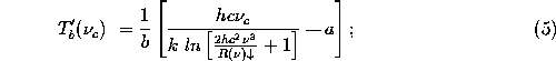
where a and b are the least-squares fit y-intercept and slope, respectively. Appendix B summarizes this approach and illustrates the associated errors.
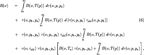
Additional absorption and radiative feedback must be accounted for if a cloud is introduced to the atmosphere. When this occurs, the atmosphere can be partitioned into layers: clear sky below the cloud, cloud layer, and clear sky above the cloud; assuming a single cloud layer. Equation 2, the clear sky RTE, would be adjusted as
where
|
| = | cloud transmissivity, from cloud base to p; |
|
| = | angular integrated cloud reflectivity; |
|
| = | cloud base pressure, hPa; and |
|
| = | cloud top pressure, hPa. |
The first three terms of
Equation 6 are an expansion of Equation 2,
whereas the last term accounts for the reflection of upwelling
terrestrial and atmospheric radiation from below the cloud.
A cloud particle size distribution outside the 50 ![]() m radius
reflectance parameterization yields a very small (see
Appendix D) change in the radiance. This
accounts for the approximation in Equation 6.
m radius
reflectance parameterization yields a very small (see
Appendix D) change in the radiance. This
accounts for the approximation in Equation 6.
The following sections discuss the individual terms of the cloudy RTE, where:
an atmospheric transmission model is used to calculate the clear
sky values; an evaluation of cloud optical properties will lead to a
cloud reflectivity term; and the RTE can be inverted to derive an
optical depth for the cloud. The final section describes a technique to
determine an estimate of the optical depth using the 9.6 ![]() m ozone band.
m ozone band.