

Next: Calculating Time-Averaged Wind
Up: Wind Profiling Method
Previous: Processing CAPPI Scans
Return to the Publications.
Return to the Index.
The wind estimate is determined from the maximum correlation peak
in three steps. First, the region with greatest weight is selected as a
global maximum correlation region.
Then, the highest peak of the global maximum region is determined.
Finally, the wind speed and direction are calculated.
The maximum correlation peak was determined
from a spatially low pass filtered correlation function
in an earlier study
[45].
The optimal filter length, however, depends on the noise level and
aerosol structure formations, which both vary with atmospheric conditions.
To reduce the number of user-adjustable parameters in the analysis,
this study uses the following approach to locate the maximum
correlation peak.
First, the global maximum correlation amplitude is found.
Then, all regions with an amplitude greater than  of the global maximum
correlation amplitude are located.
The mass m of each region is calculated by summing all
correlation amplitudes inside the region above the
  level.
The region with greatest mass
  is assumed to contain the maximum correlation peak.
The masses of the regions are also used in the
reliability analysis (see section 4.2.1).
To use information from more than one point to reduce noise,
the top of the global maximum correlation region is determined
by least-squares-fitting a two-dimensional polynomial function
to a 5 5 domain around the highest point of
the global maximum correlation region.
The maximum point of the fitted function is used as the maximum peak position
to gain sub-pixel resolution.
Sub-pixel resolution is achievable since aerosol structure formations
undergoing approximate Gaussian turbulence
[65]
lead to smooth-peaked cross correlation functions.
The fitted function is expressed as

where x and y denote coordinates in correlation plane and
 s are model parameters.
The model parameters  are solved from a
linear equation group

where  are the fit point coordinates
and
  is the cross correlation function amplitude.
The least-squares solution of the parameter vector a
in a matrix form is
[66]

where  denotes the transpose of matrix
G and
  the inverse of a square matrix.
After solving the model parameters,
the position of the maximum point
  of function
  is determined by solving equations

leading to

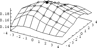
Figure 26
shows an example of the fit to the maximum CCF region.
The top of the region is wide and the
points near the local maximum have almost the same intensity.
The maximum point of the fitted function interpolates
between pixels to gain sub-pixel resolution.
The polynomial fit is less sensitive to noise than
the bicubic spline fit used in the earlier studies
[45].
The least-squares fit slightly filters the top, while
the bicubic spline may have noise-induced oscillations near
the maximum peak.

Figure 26:
The cross correlation function maximum (wire frame)
on July 28, 1989, from 12:00 to 12:03 CDT at 500 meters altitude,
fit points (diamonds), and the peak determined from the fit (rectangle).
The horizontal axes represent the distance from the maximum point in pixels
(one pixel equals 47 m).
The correlation coefficient values are plotted on the vertical axis.
The wind speed and direction are determined from the
maximum point of the fitted polynomial
representing mean movements of the aerosol structures
between the CAPPI scans.
The wind speed u and direction  are given by

where  is the time separation between subsequent volume scans.


Next: Calculating Time-Averaged Wind
Up: Wind Profiling Method
Previous: Processing CAPPI Scans
Return to the Publications.
Return to the Index.
Antti Piironen
Tue Mar 26 20:53:05 CST 1996
 of the global maximum
correlation amplitude are located.
The mass m of each region is calculated by summing all
correlation amplitudes inside the region above the
  level.
The region with greatest mass
  is assumed to contain the maximum correlation peak.
The masses of the regions are also used in the
reliability analysis (see section 4.2.1).


 5 domain around the highest point of
the global maximum correlation region.
The maximum point of the fitted function is used as the maximum peak position
to gain sub-pixel resolution.
Sub-pixel resolution is achievable since aerosol structure formations
undergoing approximate Gaussian turbulence
[
 s are model parameters.
 are solved from a
linear equation group

 are the fit point coordinates
and
  is the cross correlation function amplitude.
The least-squares solution of the parameter vector a
in a matrix form is
[
 denotes the transpose of matrix
G and
  the inverse of a square matrix.
After solving the model parameters,
the position of the maximum point
  of function
  is determined by solving equations


 are given by

 is the time separation between subsequent volume scans.