Return to the Publications.
Return to the Index.
Figure 14 illustrates HSRL and AERI optical depth measurements at Madison, WI on 17 November 1994. All derived optical depth values are shown on the graph: the solid black line represents HSRL visible optical depth; the thin, gray lines are the AERI microwindow infrared optical depths; and the dashed, black line is infrared optical depth derived from attenuation of ozone radiance due to cirrus. Calculations based on ozone attenuation are shown for completeness. A local ozone profile is not available and requires the use of the mid-latitude standard model employed by FASCOD3P. Model calculations overestimate the column ozone radiance for Madison, WI. Local data implies that scaling the FASCOD3P derived column ozone radiance below the cloud to 70 percent of the original value yields an infrared optical depth consistent with microwindow values. The proper approach requires scaling the ozone concentration rather than the radiance. Nonetheless, this approach is feasible for the optically thin ozone transmittance below the cloud base.
The HSRL and AERI microwindow optical depth data agree well in Figure 14; aside from a few points which will be discussed next. The nearly 2:1 ratio between visible and infrared optical depths is expected from theory. This occurs because the scattering cross-section is roughly two-fold larger than the absorption cross-section. The spread in AERI microwindow data as the optical depth increases is due to the index of refraction of ice spectral dependence, and will be compared to Mie theory for the statistical ensemble of points for the cases listed in Table 3.
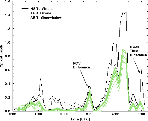
Figure 14: HSRL visible and AERI infrared optical
depth as a function of time
on 17 November 1994. The numerous thin, gray lines represent the
various AERI microwindow regions. Note the spread in the microwindow
lines as a result of the optical depth spectral
dependence. Inconsistencies in the data near 03:00 and 05:00 UTC are a
result of HSRL and AERI field of view and averaging differences.
Cirrus clouds are structured bodies that exhibit change as they are advected within the instrument's respective field of views; and is apparent in the HSRL data given in Figures 10 through 13. This provides several problems in the data inversion process: changes in cloud base and top altitude as a function of time; temporal averaging errors and dwell time differences between the instruments; and spatial averaging errors due to field of view differences between the instruments. The magnitude of these errors is determined by comparing differences in observations with model calculations and is detailed in the following paragraphs.
The AERI data inversion relies on FASCOD3P model simulations to provide the clear sky radiance and transmissivity from the surface to cloud base. The model simulated clear sky calculations must be modified according to the HSRL measured cloud base altitude changes, where the cloud base altitude can easily shift by 3 to 5 km in a period of two hours. A table of cloud base heights, based on HSRL data, is generated for each AERI data point such that the proper model output is used at the given time. However, this approach creates a secondary problem inherent to the Gamma correction that is applied to the model.
Recall that the Gamma correction provides a spectral modification to the model clear sky transmissivity. This corrects for differences relative to AERI measured clear sky radiance, primarily due to errors in the model water vapor continuum. The transmissivity correction, which is scaled by the spectral Gamma values, is not affected by the presence of clouds. However, the radiance correction is based upon a single value that represents the total clear sky column radiance, and is not Gamma corrected for a portion of the total column when clouds are present. Section 2.1.2 discussed a correction, where it was assumed that the radiance difference is due to lower atmospheric emission. The spectral bias between measured and calculated total column radiance is applied to the FASCOD3P calculated values from surface to cloud base. This accounts for the FASCOD3P radiance bias in cloudy cases where only a portion of the total atmospheric column radiance is clear. Therefore, the Gamma correction can also be applied to the clear sky radiance in an atmospheric column below the cloud.
HSRL data points are obtained roughly every 3 seconds and are averaged over 3 to 5 minute intervals to determine the optical depth. AERI data is acquired over a 3 minute dwell time, but has a nearly 4 minute dark period due to system calibration and data transfer. One obvious error results when a sudden change in the cloud optical depth occurs over a short time period, and is apparent in Figure 14. The AERI is in calibration mode at 05:00 UTC and does not observe a large change in optical depth, which is measured by the HSRL.
Discrepancies between the instruments due to data point sampling, such as the previous example, are apparent in the data. However, less obvious are the errors inherent to the averaging process for the given instrument. Spatial and temporal averaging are coupled, because the atmosphere is advected through the instrument's field of view. The effect is largest for broken clouds, where a portion of optically thick cloud would be dominated by a portion of clear sky. Structural features, such as spikes in the data due to contrails, become less identifiable in the data set as the time average is increased.
A similar effect occurs due to field of view differences, 160 ![]() rad
for the HSRL compared to 32 mrad for the AERI. This corresponds to an AERI
observed area that is more than four orders of magnitude larger than the
HSRL. The difference becomes significant for several conditions: the
HSRL is observing the edge of a cloud that is within the AERI FOV; a
small break in cloud cover occurs in the HSRL FOV, but is not
detectable within the larger AERI FOV; or the HSRL FOV is clear, but a
small band of clouds is clipping the edge of the AERI FOV. Each of
these cases would yield an AERI measured optical depth that is larger
than expected based on HSRL observations. Figure 14
illustrates a possible occurrence of this effect near 03:00 UTC. Although
the field of views were not monitored by video at this time, one would expect
this feature during a case of broken cirrus. A similar feature is not
apparent in Figure 15, where the cloud cover was noted
as uniform.
rad
for the HSRL compared to 32 mrad for the AERI. This corresponds to an AERI
observed area that is more than four orders of magnitude larger than the
HSRL. The difference becomes significant for several conditions: the
HSRL is observing the edge of a cloud that is within the AERI FOV; a
small break in cloud cover occurs in the HSRL FOV, but is not
detectable within the larger AERI FOV; or the HSRL FOV is clear, but a
small band of clouds is clipping the edge of the AERI FOV. Each of
these cases would yield an AERI measured optical depth that is larger
than expected based on HSRL observations. Figure 14
illustrates a possible occurrence of this effect near 03:00 UTC. Although
the field of views were not monitored by video at this time, one would expect
this feature during a case of broken cirrus. A similar feature is not
apparent in Figure 15, where the cloud cover was noted
as uniform.
An additional factor regarding data acquisition which should be noted is the observation direction of each instrument. The HSRL is tilted 4 degrees from zenith to prevent specular reflection in the return signal. This corresponds to a 60 mrad offset from zenith, which is greater than the 32 mrad field of view of the AERI. Thus, each instrument will observe completely different scenes unless care is taken to properly align the systems. The instruments were only roughly aligned for the given case study.
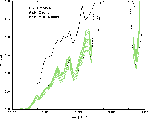
Figure 15: HSRL visible and AERI infrared optical depth as a function of time
on 9-10 November 1995. The cloud becomes opaque between 01:30 and 02:30
UTC, signified by an optical depth greater than 3.0.
Optical depth data for the cirrus cases listed in Table 3 were combined and compared against HSRL measured values. This was performed for each microwindow and interpreted with a Least-Squares fit. HSRL averaged data was extrapolated to be similar with AERI times to account for differences in sampling. Values were also limited to optical depths of less than 2 in the visible, which falls well below the HSRL upper limit of 3. Infrared optical depths were limited to 1.6. Figure 16 illustrates the infrared optical depth as a function of cirrus cloud radiance. The IR optical depth gradually increases to a value of 1.6, where it doubles to 3.0 with an additional 25 percent increase in cloud radiance. Above this value, a 5 percent increase in cloud radiance yields a large increase in the optical depth. These calculations suggest that OD values above 3.0 are very uncertain, thus these clouds are assumed to be opaque.
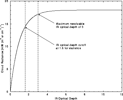
Figure 16: Infrared optical depth as a function of cloud radiance. An AERI
IR optical depth cut-off value of 1.6 was used when comparing
against HSRL visible data. Small changes in cloud radiance yield a
large increase in the cloud optical depth for IR optical depths
greater than 3, and the cloud is considered opaque.
Figure 17 shows the results of
this technique for the microwindow located at 862 cm![]() . The slope is
representative of the visible to infrared optical depth ratio,
. The slope is
representative of the visible to infrared optical depth ratio,
![]() , and was
determined to be 1.790 given roughly 70 data
points. Figure 17 comprises data from the entire
cirrus case study, however the scatter about the Least-Squares fit remains
large. This eliminates the ability to
determine similar results for a single case. Table 4 lists
, and was
determined to be 1.790 given roughly 70 data
points. Figure 17 comprises data from the entire
cirrus case study, however the scatter about the Least-Squares fit remains
large. This eliminates the ability to
determine similar results for a single case. Table 4 lists
![]() for the remainder of the microwindow regions using this approach.
Results from the other technique detailed in the last portion of
Section 2.2.4, which iterates a solution for
for the remainder of the microwindow regions using this approach.
Results from the other technique detailed in the last portion of
Section 2.2.4, which iterates a solution for
![]() , are given in Section 4.2.
, are given in Section 4.2.
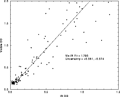
Figure 17: Comparison of HSRL visible and AERI 862 cm![]() microwindow infrared
optical depth for the cirrus cases listed in Table
3. Least-squares fit slope yields visible to IR optical
depth ratio of 1.790, with greater than 4 percent uncertainty.
microwindow infrared
optical depth for the cirrus cases listed in Table
3. Least-squares fit slope yields visible to IR optical
depth ratio of 1.790, with greater than 4 percent uncertainty.
|
Microwindow | |
Microwindow | |
| 773.12 788.55 811.21 820.13 831.70 845.69 862.32 875.10 894.14 902.10 | 1.8523 1.7602 1.8264 1.7300 1.7433 1.8828 1.7897 1.7895 1.7510 1.7570 | 934.88 962.37 991.78 1080.97 1095.68 1115.21 1128.71 1145.34 1159.56 | 1.8528 1.9176 2.0572 2.1313 2.0944 2.0344 2.0226 1.9964 2.0005 |
A number of additional errors, not related to the instrumental data acquisition characteristics described previously, can contribute to the scatter plot shown in Figure 17. The primary source of error in the visible is due to multiple scattering; whereas uncertainties in radiosonde measurements and misrepresentation in the model simulated water vapor continuum are the largest factors in the infrared. Of course, instrumental spatial and temporal differences are always a significant factor. Application of the Gamma correction, Section 2.1.2, reduces the errors associated with the water vapor continuum.
A significant portion of the HSRL backscattered signal can be
attributed to multiple scattering, despite the narrow HSRL field of
view. Multiple scatter data on 9-10 November 1995 suggests that as
much as 20% of the aerosol signal is due to multiply-scattered
return, while using the 160 ![]() rad FOV (Eloranta
and Piironen, 1996). This effect is
a function of optical depth; and it depends on the particle size, where
the forward scatter diffraction peak narrows as the particle
size increases. A portion of the forward diffraction peak is narrow enough to
remain within the HSRL field of view. Thus, although the photon has
experienced extinction through diffraction about the particle, it
remains with the original pulse and may contribute to the return
signal if backscattered by a second particle. This effect yields a
larger than expected return signal, corresponding to a smaller than expected
optical depth near cloud base. This is shown in Figure 18 as a
function of the backscatter cross-section, relative to the observed
molecular signal, for both the corrected and uncorrected cases.
rad FOV (Eloranta
and Piironen, 1996). This effect is
a function of optical depth; and it depends on the particle size, where
the forward scatter diffraction peak narrows as the particle
size increases. A portion of the forward diffraction peak is narrow enough to
remain within the HSRL field of view. Thus, although the photon has
experienced extinction through diffraction about the particle, it
remains with the original pulse and may contribute to the return
signal if backscattered by a second particle. This effect yields a
larger than expected return signal, corresponding to a smaller than expected
optical depth near cloud base. This is shown in Figure 18 as a
function of the backscatter cross-section, relative to the observed
molecular signal, for both the corrected and uncorrected cases.
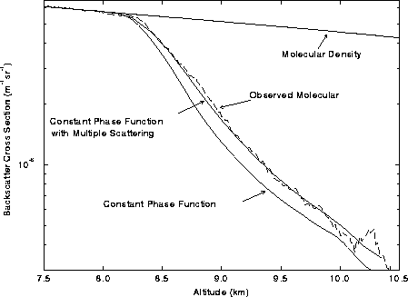
Figure 18: HSRL backscatter cross-section as a function of altitude for data
taken between 23:55 and 00:03 UTC 9-10 November 1995. Shown are the
observed molecular backscatter cross-section, dashed line; corrected
backscatter cross-section based on a constant phase function, lowest
line; the adjusted backscatter cross-section based on a constant phase
function and multiple scatter model, solid line near dashed line; and
the observed molecular density profile.
Figure 18 illustrates the molecular density profile,
determined from radiosonde measurements, relative to the molecular backscatter
cross-section measured by the HSRL (dashed line) for data taken
between 23:55 and 00:03 UTC on 9-10 November 1995. Also shown is the
corrected backscatter cross-section profile based on a constant phase
function fit using diffraction theory to match the top of cloud
measurements (Eloranta and Piironen, 1996). The difference between the HSRL
measured data and constant phase function corrected data is assumed to
be due to multiple scattering. Application of the multiple scattering model
(Eloranta and Shipley, 1982; Eloranta, 1993) to the data indicates the
difference to be a
result of multiple scattering from 56 ![]() m radius spheres, with
similar cross-sectional area as ice crystals. It will be shown that
this size is consistent with Mie theory for the set of cirrus data
cases given in Table 3.
m radius spheres, with
similar cross-sectional area as ice crystals. It will be shown that
this size is consistent with Mie theory for the set of cirrus data
cases given in Table 3.
The maximum expected uncertainty in the radiosonde measurements were given in Table 2: 0.2 K and 2 K for temperature and dewpoint temperature, respectively. However, additional radiosonde errors occur as a result of spatial differences between the AERI and the radiosonde, and from changes in the atmospheric temperature structure as a function of time. These uncertainties translate into errors in the FASCOD3P calculated radiance.
The radiosonde drifts with the mean wind as it rises, reaching upwards of 200 km from the UW launch point. However, it was already shown that the radiance contribution above 9 km is negligible. This implies that the spatial drift is a concern only during the first 9 km of ascent. Furthermore, the lowest 3 km of the atmospheric column contributes over 80 percent of the measured radiance within the microwindows. A radiosonde ascent rate of 4.5 m per second would reach this altitude within 15 minutes, traveling less than 10 km from the launch point during normal wind conditions. Therefore, discrepancies caused by spatial errors are small compared to the instrument uncertainties. A frontal passage would be an exception to this argument, where a strong contrast in temperature and dewpoint temperature exists over a similar range. This is not a factor for the cirrus cases used in this thesis.
AERI data acquisition may continue for several hours after the release of a radiosonde, measuring the column radiance from an atmosphere with a modified temperature structure with respect to the radiosonde profile. A pair of radiosondes were released within 3 hours, 00:00 and 03:00 UTC, from the UW on 17 November 1994 to determine the effect of atmospheric changes over a typical data acquisition period. The temperature and dewpoint temperature profiles for each radiosonde are given in Figure 19. Both cases illustrate the constrained dewpoint temperature profile lower bounds, which are a result of very dry conditions. This occurs because a measured relative humidity of exactly zero is set to a small value above zero to avoid a singularity. The radiosonde release times of 00:00 and 03:00 UTC occured after sunset. The data suggests a decrease in the boundary layer thickness and decrease in surface temperature, which is consistent with subsidence above the boundary layer after sunset. FASCOD3P calculations were performed to determine the change in atmospheric column radiance for each case. Assuming the differences can be attributed to advection and atmospheric heating rates, the changes in radiance caused by this effect can be added to the expected radiative error due to radiosonde instrument uncertainty.
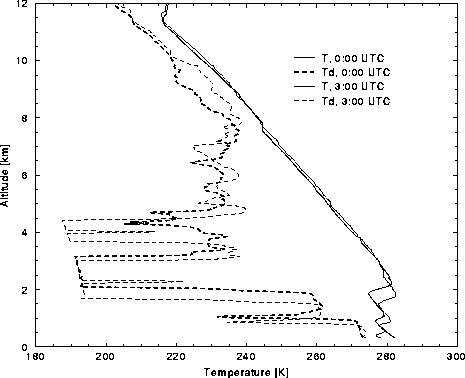
Figure 19: Comparison of temperature (solid lines) and dewpoint temperature
(dashed lines) data for radiosondes launched from the UW at 00:00
(heavy lines) and 03:00 (thin lines) UTC on 17 November 1994. Note the
decrease in surface temperature and decrease in boundary layer
thickness that occurs between 00:00 to 03:00 UTC.
Radiance errors associated with instrumental and atmospheric uncertainties in the radiosonde measurements are given in Figure 20. The upper portion of Figure 20 illustrates the FASCOD3P radiance difference due to changes in the atmospheric temperature and dewpoint temperature structures indicated in Figure 19 (lower line), and due to uncertainties in the radiosonde measurements (middle line). The total error (upper line) is the combined contribution. The lower portion of Figure 20 gives the percent error in cloud radiance, derived from the AERI data on 17 November 1994, for a measured IR optical depth of 0.5, based on these discrepancies. Note the advantage of high spectral resolution measurements, where the radiance errors are smaller in the microwindow regions than on an absorption line.
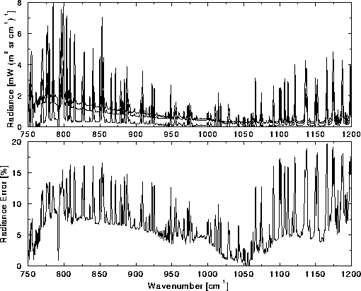
Figure 20: Upper figure shows expected radiance error due to atmospheric
changes over a 3 hour period (lower line), refer to Figure 19;
error due to expected uncertainties in the radiosonde measurements
(middle line), refer to Table 2; and combined radiance error
assuming both circumstances (upper line). The lower figure illustrates
the percent deviation in cloud radiance, given the above
data, for AERI data on 17 November 1994; where the
resultant error is calculated for an AERI measured IR optical depth of 0.5
The spectral radiance errors shown in Figure 20 can be used to
determine the uncertainties in AERI derived infrared optical
depths. Data from 17 November 1994 was inverted using the radiance
uncertainty limits to calculate bounds on the infrared optical
depths. Figure 21 illustrates the results for a pair of
microwindow regions for this data case. The upper figure shows the
1080 cm![]() microwindow, representing the most transparent microwindow;
whereas the lower figure gives the 810 cm
microwindow, representing the most transparent microwindow;
whereas the lower figure gives the 810 cm![]() results,
representing the most opaque microwindow. Error bounds are given by
the dotted lines, such that the shaded portion yields the
optical depth uncertainty. The bold, solid line indicates the
measured infrared optical depth.
results,
representing the most opaque microwindow. Error bounds are given by
the dotted lines, such that the shaded portion yields the
optical depth uncertainty. The bold, solid line indicates the
measured infrared optical depth.
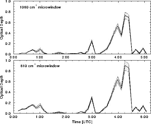
Figure 21: AERI measured optical depth uncertainty for data acquired 17
November 1994. Upper figure indicates 1080 cm![]() measured optical
depth (bold, solid line) and its uncertainty (shaded region) given
radiosonde radiance error illustrated in
Figure 20. Lower figure shows 810 cm
measured optical
depth (bold, solid line) and its uncertainty (shaded region) given
radiosonde radiance error illustrated in
Figure 20. Lower figure shows 810 cm![]() microwindow
data. These regions were chosen because the represent the microwindow
optical depth extrema.
microwindow
data. These regions were chosen because the represent the microwindow
optical depth extrema.
Data given in Table 4 was spectrally compared to Mie
theory, assuming spherical ice particles, where the index of refraction for
ice was taken from Warren (1984). Calculations are based on a
Hansen distribution, Equation 12, using an effective
radius of 25, 50, and 100 ![]() m. The results and imaginary index of
refraction are illustrated in Figure 22. The
theoretical results compare the scattering efficiency,
m. The results and imaginary index of
refraction are illustrated in Figure 22. The
theoretical results compare the scattering efficiency, ![]() ,
near the lidar wavelength relative to the absorption efficiency,
,
near the lidar wavelength relative to the absorption efficiency,
![]() , for a series of spectral regions in the infrared. The
experimentally derived results exhibit a
trend similar to the Mie calculations near a 50
, for a series of spectral regions in the infrared. The
experimentally derived results exhibit a
trend similar to the Mie calculations near a 50 ![]() m effective
radius. This is consistent with multiple scattering measurements on
9-10 November 1995, Figure 18,
where a diffraction theory fit to the data
estimated particles with an area equivalent to 56
m effective
radius. This is consistent with multiple scattering measurements on
9-10 November 1995, Figure 18,
where a diffraction theory fit to the data
estimated particles with an area equivalent to 56 ![]() m radius
spheres (Eloranta and Piironen, 1996). It will be shown in
Section 4.2 that the experimental
results improve when using an HSRL weighted cloud extinction cross-section.
m radius
spheres (Eloranta and Piironen, 1996). It will be shown in
Section 4.2 that the experimental
results improve when using an HSRL weighted cloud extinction cross-section.
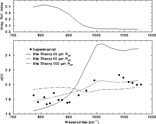
Figure 22: Spectral comparison of experimentally derived ![]() against Mie theory for various particle size
distributions. Upper plot illustrates imaginary index of refraction
used in Mie calculations, taken from Warren (1984). The cross-over
point, near 920 cm
against Mie theory for various particle size
distributions. Upper plot illustrates imaginary index of refraction
used in Mie calculations, taken from Warren (1984). The cross-over
point, near 920 cm![]() , in the Mie theory
curves suggests that this
spectral region is least sensitive to particle size.
, in the Mie theory
curves suggests that this
spectral region is least sensitive to particle size.
An interesting feature of Figure 22 occurs near 920
cm![]() , where the Mie theory lines overlap. This is the
transition point
from strong to weak absorption, with increasing wavenumber. Data
outside this region is more sensitive to particle
size. Figure 22 suggests that a
visible to infrared ratio near 1.9, representing 920 cm
, where the Mie theory lines overlap. This is the
transition point
from strong to weak absorption, with increasing wavenumber. Data
outside this region is more sensitive to particle
size. Figure 22 suggests that a
visible to infrared ratio near 1.9, representing 920 cm![]() data, would
be least dependent on changes in particle size.
data, would
be least dependent on changes in particle size.
As the imaginary index of refraction increases, the particle becomes
an efficient absorber; such that the ratio of visible to infrared
optical depths approaches a limit as the particle size
increases and becomes opaque. In the realm of weak absorption, the
particle is not
opaque and produces extinction that is proportional to the product of
the absorption coefficient and particle volume (Liou et al.,
1990); where the
absorption coefficient is proportional to the product of the imaginary
index of refraction and the wavenumber. For strong absorption, the
extinction is dependent on the particle area. The change in the
imaginary index of refraction of ice, shown in Figure 22, is
large enough across the AERI microwindow range to visualize this effect.
Wavenumbers between 1000 and 1150 cm![]() are in the realm of weak absorption
and exhibit a large dependence on particle size. As the absorption
increases, 800 to 900 cm
are in the realm of weak absorption
and exhibit a large dependence on particle size. As the absorption
increases, 800 to 900 cm![]() , the lines are
closer together.
, the lines are
closer together.