


When fractional cloud coverage increases, echoes from the clouds can bias the CBL depth estimate by dominating the variance. In such cases, the variance maximum represents the altitude of maximum cloud echo variability instead of the convective boundary layer mean depth. In this study, the automatic method for determining CBL mean depths in the presence of a few low-altitude clouds is similar to the clear air case described in the previous section, except that the shadowed regions behind clouds are removed from the computation of the horizontal variance. This prevents bias due to cloud shadows, which do not add information about the aerosol distribution. However, when cloud coverage increases, the results may be biased by cloud echoes. Therefore, CBL mean depths above the cloud base must be interpreted with caution.
Figure 9 presents a comparison of manually and automatically determined CBL mean depths from the 1989 FIFE experiment when the cloud coverage was less than 10%. The manual and automatic estimates generally correlate well. When the CBL mean depth is below 200 m, the lidar images show only the tops of the plumes. This may bias both manual and automatic results to higher than the actual CBL mean depth. Therefore, the lowest CBL estimates must be used with caution. Otherwise, the deviations are mostly due to under-sampling of an undulating CBL top in the manual method, which causes typically 100--200 m variations in the estimates. Although the manual estimates vary more than the automatic estimates, the manual method provides better sampling coverage than any point measuring system. Boxes a-- c show some of the most extreme discrepancies between the manual and automatic methods. Measurements in these boxes were reanalyzed to explain the scatter in the plot. Box a marks a CBL depth estimate which was due to under-sampling of a strongly undulating CBL top. Box b marks points for which a haze layer just above the CBL was manually misinterpreted as the CBL top. The haze layer was difficult to separate from the CBL top in manual interpretation, since the haze layer and CBL top had similar backscatter signal strengths and only a narrow layer of clearer air separated the layers. Box c marks a point which was hard to determine using the manual method due to low contrast between boundary layer aerosols and free air. After reinterpretation, the manual estimates were within 100 m of the automatic measurements.

Figure 9: Automatically vs. manually
determined convective boundary layer mean depth with low cloud coverage
from July 26 to August 11, 1989.
Boxes a and c mark points where the CBL mean depth was difficult
to determine using the manual method due to low contrast between the
boundary layer aerosols and free air; box b marks points which
were manually misinterpreted.
After reinterpretation, the
manual estimates in these boxes were within 100 m of the automatic
estimates.
When convective clouds dominate the boundary layer structure, the definition of a CBL mean depth becomes unclear and the previously presented convective boundary layer mean depth determination is invalid. For example, near a thunderstorm cloud with a cloud top at 10 km, the local boundary layer would be 5 km by the definition adopted here. In the presence of low clouds, the cloud base and cloud top altitudes are presented. In these cases, the values of the mean depth must be interpreted with caution. Figure 10 presents an RHI scan along with a signal variance profile and CBL mean depth estimate. Echoes from clouds cause a strong backscatter signal variance. Clouds make automatic determination of the CBL mean depth uncertain. However, Figure 9 suggests the automatic CBL mean depths are reliable if the fractional cloud coverage does not exceed 10%. When more low-altitude clouds are present, the manual inspection of the RHI scans provides more reliable CBL mean depth estimates, although it is very time consuming.
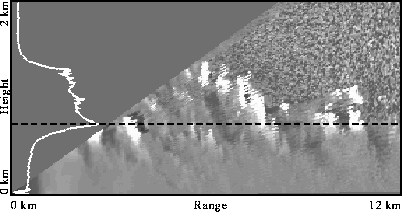
Figure 10: An RHI scan, the variance of the filtered backscatter
signal as a function of altitude (white curve),
and the CBL mean depth estimate (black dashed line)
on August 2, 1989, at 12:00 CDT.
Bright structures on the RHI scan represent cloud echoes.
In this case, clouds make estimation of the CBL mean depth uncertain.