

Next: Data Normalization
Up: Cirrus Cloud Optical and
Previous: Conclusion
Return to the Publications.
Return to the Index.
To correctly calibrate the VIL data, the system limited data points had to be
removed from the data set. At far ranges the backscattered radiation can not
be separated from the system noise because the VIL signal decreases due to
the range squared dependence and attenuation.
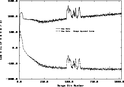
When the VIL raw data is corrected for the range squared
dependence, the places where the VIL signal increases monotonically
as a function of the
range is where the signal could not be separated from the noise as seen in
Figure 15. This limit of
detectability occurs where the VIL signal
starts to increase with range around bin 250. The large increase in the
signal around the range bin 500 was the result of radiation backscattered
from a cirrus cloud.
To remove the noise dominated points, the points where the raw signal
was within the noise regime had to be determined. At far ranges, the raw
backscattered signal becomes linear with range when the backscattered
power is plotted on a natural log scale. This was a result of both the
attenuation of the transmitted pulse in the atmosphere and the range
squared decrease of the signal. Shot noise occurs along with the raw signal.
If the shot noise was
random, as expected, then the noise should occur as a Gaussian distribution
about the raw data. This would not affect the slope
of the VIL data with range in Figure 15.
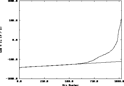
So, if the VIL raw data was sorted according to their magnitudes and
replotted on a log-linear plot, then the signal which was small
and could not be separated from the noise would appear as a straight
line at the lower signal magnitudes (Figure 16).
This process was applied to each VIL raw profile where the VIL backscatter
signal was sorted according to their magnitudes. The sorted values were
approximated using a straight line median fit.
The straight line median fit was first applied to the whole sorted
profile. The points occurring above the fit had large signal backscatter
and were remove from the sorted set. The remaining sorted points
were then refitted using a straight line median fit. After a number of
successive fits, where a chosen threshold was met, the remaining
points consisted only of the small signal values which could not be
separated from the noise (they appear as a straight line
in Figure 16). These noise points were
discarded from the original data set. For the shot used in
Figure 15 and Figure 16, over one half of the data
points had to be discarded. The remaining data
points are the signal backscattered by aerosols and molecules
in the atmosphere.

Figure 15: Removal of the noise points from the VIL raw data. The x-axis is
the range bin number and the y-axis is 128  ln (P / E) for the raw
data and 128
  ln (P * R * R / E) for the range squared corrected
raw data. The solid line is the range squared corrected VIL profile. The
long dashed line is the VIL raw data profile.

Figure 16: Removal of the noise points from the VIL raw data. The x-axis
is the sorted bin number. The y-axis is 128  ln (P / E). The
solid line is sorted VIL raw data (sorted according to magnitudes).
The dashed line is the straight line median best fit
to the sorted noise points.


Next: Data Normalization
Up: Cirrus Cloud Optical and
Previous: Conclusion
Return to the Publications.
Return to the Index.
Antti Piironen
Thu Apr 11 08:27:54 CDT 1996

 ln (P / E) for the raw
data and 128
  ln (P * R * R / E) for the range squared corrected
raw data. The solid line is the range squared corrected VIL profile. The
long dashed line is the VIL raw data profile.


 ln (P / E). The
solid line is sorted VIL raw data (sorted according to magnitudes).
The dashed line is the straight line median best fit
to the sorted noise points.