Next: About this document Previous: Conference papers

Introduction

In this paper, both horizontal components of the wind vector are measured with 250 m spatial resolution over a 6 by 10 km area. These are derived using 2-dimensional cross-correlations computed between a series of aerosol backscatter images recorded with the University of Wisconsin Volume Imaging Lidar (VIL).

The VIL is designed to provide high spatial and temporal resolution images of atmospheric structure. It employs a m laser operating at a repetition rate of 100 Hz, 0.5-m diameter scanning optics, and a fast data acquisition system to generate two- and three-dimensional images. Under typical conditions, the system records data to a range of 18 km with a range resolution of 15 m. The data system records profiles without averaging. Approximately 1 G-byte of data is recorded per hour of operation.

This paper analyzes repeated azimuthal scans made with the lidar elevation angle set near zero. A typical scan covered an azimuthal sector of and provided lidar profiles at increments. The full back-and-forth scan was repeated at s intervals.

Wind Calculations

We have previously developed algorithms to measure vertical profiles of the horizontal wind from a series of volumetric lidar images of aerosol structure (Schols and Eloranta 1992, Piironen and Eloranta, 1995). These provide a single wind vector for each altitude representing the mean wind averaged over the km area of a typical scan. In this paper, these algorithms are modified to provide a vector wind field with a 250 m spatial resolution. Correlations are computed between square image segments which are 250 meters on a side. Correlations are computed between every other scan so that left-moving and right-moving scans are always paired with the same scan direction and thus the time interval between laser profiles in each part of successive images is s. Because the winds were as large as 9 m/s, the wind advected aerosol structures by up to 225 m between scans. This created noise in the cross correlation calculation because most of the structure seen in the first image was advected out of the image area before the next scan. To minimize this problem, the second image in each correlation pair is selected from a position displaced downwind of the first image by the distance the structure is expected to move between scans. This allows the correlation to take place with approximately the same air mass that was present in the first image. The displacement of the image position is added to the displacement of the correlation peak to compute the wind vector. The a priori wind vector required to compute the displacement of the second image is computed by first generating a wind field with 500 m spatial resolution where the advection distance is a smaller fraction of the image size.

Figure 1 shows the wind field computed from data acquired 5 m above the surface of Lake Michigan as cold air ( C) passed over C water. Figure 2, which presents North-South averages, shows the acceleration and veering of the wind as it leaves the shore. The wind shadow in the lee of the coastline is clearly visible. A careful examination of figure 1 shows that the wind shadow length varies with position. This reflects variations in the topography and surface roughness along the shore. The error bars in figure 2 were computed from the variance of the values contributing to each north-south average; with the errors set equal to the square-root of the variance divided by the square root of the number of points contributing to the average (24 points in this case). These tend to underestimate the true error by failing to include systematic errors while at the same time tending to overestimate the errors because the true geophysical variability is included in the calculated variance. The estimated errors in the North-South average wind speed and direction are cm/s and respectively, while for the individual wind measurements shown in figure 1, the estimated errors are cm/s and for the speed and velocity respectively.

This paper will also present divergence and vorticity fields computed from the vector winds.

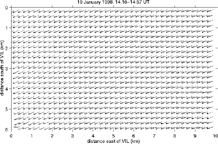
Figure 1. Wind vectors computed from 240 PPI scans 5 m above lake Michigan during a cold air outbreak between 14:15 and 14:57 UT on January 10, 1998. The shore line roughly parallels the left edge of the figure. Meteorological wind barbs are presented with single barbs and triangles indicating 1 m/s and 5 m/s respectively.

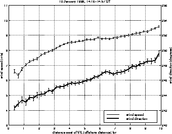
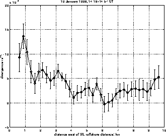
Figure 2. Average wind speed, direction (left-panel) and divergence (right-panel) as a function of distance from the shore between 14:15 and 14:57 UT on January 10, 1998. The acceleration and veering of the wind with offshore distance are clearly seen. This plot is computed from a north-south averaging of the data shown in figure 1.

References

• Schols, J. L., and E. W. Eloranta, 1992: The calculation of area-averaged vertical profiles of the horizontal wind velocity from volume imaging lidar data ., J. of Geophys. Res., 97, 18395-18407.

• Piironen, A. and E. W. Eloranta, 1995: An accuracy analysis of the wind profiles calculated from Volume Imaging Lidar data, J. of Geophys. Res., 100, 25559-25567.