


We are running the University of Wisconsin's scalable non-hydrostatic modeling system (Tripoli 1992) to simulate the leading edge of a lake-induced CBL. The model is a computationally efficient, elastic, fully non-Boussinesq grid-point model which includes enstrophy conservation.
For the work presented here, which represents our first attempts to simulate the lake-induced CBL, the model was run three times with horizontal resolutions of 10, 25 and 50 m. All of the simulations used a 0.25 s time-step and a vertical resolution of 1 m at the surface which increased at a rate of 1.1*dz until a resolution of 50 m was obtained (at about 450 m.) All simulations used 140x70x80 grid-points. The surface of the western 40 grid-points of each domain was snow-covered at air-temperature and the remaining surface was water at a temperature of 279 K.
The model was initialized with horizontally homogeneous initial conditions as prescribed by a radiosonde sounding 10 km upwind (figure 3). This profile of temperature, dew point and wind is maintained along the upwind (inflow at western wall) of the domain. Cyclic (periodic) boundary conditions are implemented along the northern and southern walls of the domain. An open boundary condition is maintained along the eastern wall (outflow). A Rayleigh absorbing layer of 16-points with a minimum dissipation time of 10 s was used at the top of the model. For these runs a geostrophic and hydrostatic reference state is assumed. Subgrid-scale turbulence parameterization is a buoyancy enhanced eddy-viscosity closure similar to that of Tripoli and Cotton (1982). Heat, moisture and momentum are transferred from the surface to the lowest layer of the model using standard bulk mixing theory. The model solves for saturation and cloud water diagnostically and the steam fog is produced as the result of supersaturation assuming conservation of total water mixing ratio and entropy.
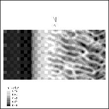
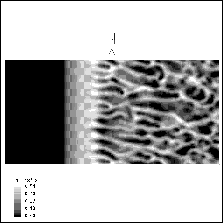
The simulation with 50-m horizontal resolution, which has a horizontal domain of 7.0 by 3.5 km, produces a homogeneous region of steam-fog along the coastline out to approximately 1.5 km offshore where linear rolls form. The image shown in figure 4 is from 30 minutes after the beginning of the simulation---long after parcels entering the upwind edge of the domain would have traversed the full east-west distance of the domain. The flow near the surface veers with increasing offshore distance. At the downwind edge of the domain, the CBL depth has grown to approximately 600 m. When streamlines of the horizontal flow (such as those in figure 6) are superimposed on the condensed water field, the bands of steam-fog lie in regions of convergence and upward motion.
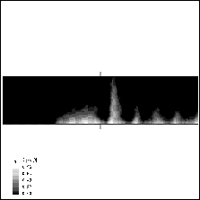
Figure 5 shows an east-west vertical slice of the lowest 15 grid-points at 30 minutes in the simulation. This image ranges from the surface to 26.2 m above the lake and is 7 km wide. The image shows the upward-sloping leading edge of the homogeneous band of steam-fog shown in figure 4 and some narrow columns of steam-fog rising from the surface of the lake. These features, which would be visible wisps of steam fog in reality, can be compared to the very bright spots along the bottom edge of the RHI shown in figure 2. The narrow columns of scattering which sometimes extend to the top of the 500-m deep mixed layer in figure 2 are composed of visible steam fog just above the surface and hygroscopically swollen aerosols at the remaining levels.
The 25 m and 10 m horizontal resolution simulations also use domains
with 140x70x80 grid-points, and thus cover less area than the 50 m
grid. The 25 m grid covers 3.5 by 1.75 km and the 10 m grid covers 1.4
km by 700 m. Both of these simulations produce a homogeneous region of
steam-fog immediately downwind of the shoreline followed by linear
rolls. Nine roll circulations set up in the 50 m grid ( = 420
m); approximately 12 in the 25 m grid (
= 420
m); approximately 12 in the 25 m grid ( =160 m), and 18 in the
10 m grid (
=160 m), and 18 in the
10 m grid ( = 40 m). The 50 m grid appears to preserve these
roll structures downstream for a much greater proportion of the grid.
Downstream of the rolls, a braided or more cellular appearing pattern,
can be seen in all three simulations. The dependence of the structure
on resolution warrants further investigation.
= 40 m). The 50 m grid appears to preserve these
roll structures downstream for a much greater proportion of the grid.
Downstream of the rolls, a braided or more cellular appearing pattern,
can be seen in all three simulations. The dependence of the structure
on resolution warrants further investigation.
All the images shown here are frames extracted from high-resolution color animations. These MPEG movies can be downloaded from our website at http://lidar.ssec.wisc.edu.